          V1         V2         V3
1  0.4814018  0.7468954 -1.4401043
2 -0.8309668 -0.6558851  1.5983829
3  0.2360548  0.8199547  1.8496925
4  0.3685305  0.9678467 -1.1387934
5 -0.5266293  0.3336697 -0.0650335
6 -0.2464255 -0.5563491 0.8534258Factor Models Primer
Factor models seek to distill often high dimensional data into a set of underlying or latent factors that capture much of the original variation in the data.
We say the data, \(X\), follows a factor structure if:
\[ \begin{align} \underset{(T \times n)}{X} = \underset{(T \times r)}{F} \underset{(r \times n)}{\Lambda^{*'}} + \underset{(T \times n)}{e} \end{align} \]
where there are
\(T\) rows (observations),
\(n\) columns (variables), and
\(r\) factors. And we can refer to
\(\lambda_{ik}^*\) as the entry in \(\Lambda^{*}\) in the \(i\)th row and \(k\)th column
This \(\lambda_{ik}^*\) shows how factor \(k\) is related to, or “loads onto,” variable \(i\). Note that the \(k\)th column of \(\Lambda^*\) will be referred to as \(\lambda_k^*\).
We assume that the number of underlying factors can be learned from the data (e.g. following the procedure in Bai and Ng (2002) or Ahn and Horenstein (2013)).1 Next, we’re interested in estimating the loading matrix \(\Lambda^*\), which shows how the factors are related to the data matrix \(X\).
Problem: Rotational Indeterminacy
However, there is no unique estimate of \(F\) and estimate of \(\Lambda^*\) that satisfies the equation above.
To illustrate, let \(H\) be any nonsingular \(r \times r\) matrix. We can define an alternative loading matrix \(\Lambda^0 = \Lambda^* (H')^{-1}\) and alternative factors \(F^0 = FH\), and it follows that
\[ \begin{align} X & = F^0 \Lambda^{0'} \\ & = FH (H^{-1'})' \Lambda^{*'}\\ & = FH H^{-1} \Lambda^{*'} \\ & = F \Lambda^{*'} \end{align} \]
Hence \((F^0,\Lambda^{0'})\) and \((F,\Lambda^*)\) are observationally equivalent. This is referred to as rotational indeterminacy and makes interpretation of any estimate of the loading matrix delicate. Each arbitrary rotation \(H\) will result in an alternate interpretation of how the factors and variables are related. But we are interested in the true relationship, \(\Lambda^*\). So how can we recover the true interpretation?
Solution: Use Sparsity
The key idea in Freyaldenhoven (2025) is that assuming a sparsity pattern in the true loadings matrix \(\Lambda^*\) solves the issue of rotational indeterminacy since the sparsity pattern is not invariant to rotations. Intuitively, any rotation (or linear combination) of a sparse loading vector will be less sparse.
To see this, note that PCA gives us estimates that are asymptotically a linear combination of the true loadings vectors. That is, we can obtain principal component vectors in the columns of \(\Lambda^0\) such that
\[ \begin{align} \Lambda^0 = \Lambda^*(H^{-1})' + \epsilon \end{align} \] where \(H\) is a nonsingular \(r \times r\) matrix and \(\epsilon\) is ``small’’.
Thus, \(\Lambda^0\) is (close to) a linear combination of \(\Lambda^*\). However, even if \(\Lambda^*\) is sparse, linear combinations of the sparse loadings in \(\Lambda^*\), such as \(\Lambda^0\), are generally not sparse.
Conversely, \(\Lambda^*\) is also (close to) a linear combination of \(\Lambda^0\). Thus, there must be a linear combination of \(\Lambda^0\) that is sparse. This sparse linear combination of \(\Lambda^0\) will be our estimator for \(\Lambda^*\).
Recovering Sparsity
Now, how do we find this sparse linear combination of loading vectors?
A simple approach would be:
- Take the principal components estimator as starting point to obtain \(\Lambda^0\)
- Find loadings \(\Lambda^*\) equal to the rotation of \(\Lambda^0\) that minimizes the number of non-zero elements (the \(l_0\) norm) in the loading vectors
Unfortunately, the \(l_0\) norm is infeasible to optimize over in practice. To see why, let’s examine the figure below. The distance from the origin to each red point depicts the \(l_0\) norm of points along the unit circle. The blue points depict the \(l_1\) norm and the gray points depict the \(l_2\) norm. In the \(l_2\) case, these distances remain constant as we traverse the circle.
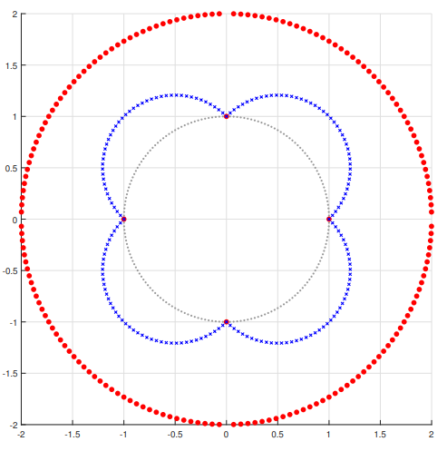
The \(l_0\) norm directly computes the number of nonzero elements, shown by the red points. At (1, 0), (0, 1), (-1, 0) and (0, -1), these are a distance of 1 away from the origin. The remaining red points are a distance of 2 away from the origin corresponding to the 2 nonzero elements in all other points along the unit circle. Since the blue and red dots coincide at the above four points, the \(l_1\) norm is minimized at the same points as the \(l_0\) norm. But the \(l_1\) norm has a smooth descent to these minima compared with the discontinuities of \(l_0\) norm around these minima. This makes the \(l_1\) easier to minimize.
Thus, to maximize sparsity we minimize the \(l_1\) norm instead of the \(l_0\) norm.
Objective Function
Formally, using the \(l_1\) norm, our objective function becomes
\[ \begin{align} \min_R ||\Lambda^0R||_1 \end{align} \] such that \(R\) is nonsingular and \(||r_k||_2 = 1\) where \(r_k\) is a row in \(R\). This keeps the length of each loading vector fixed, ensuring we look only at rotations of each initial loading vector. Since the length remains constant, we can transform this constrained optimization problem into an unconstrained one by converting to polar coordinates. For example, in the case of two factors, in the constrained version we want to find weights \(w_1, w_2\) that minimize
\[ || w_1 \lambda_1^0 + w_2 \lambda_2^0 ||_1 \quad s.t. \quad w_1^2 + w_2^2 = 1. \] In spherical coordinates, this amounts to finding an angle \(\theta\) that minimizes
\[ ||\lambda_1^0 \cos \theta + \lambda_2^0 \sin \theta ||_1. \]
A simple example
Let’s consider an example we can visualize fully: we’ll use the following simulated data that has three columns (\(n = 3\)) and suppose we know that there are two factors, \(r = 2\). Below only the first 6 of 224 total rows are printed.
Let the true loadings matrix, \(\Lambda^*\) have 2 columns and 3 rows. As we can see there is a sparsity pattern in the matrix with the first factor affecting only the first column and the second factor affecting the second and third columns of \(X\).
  loadings_1 loadings_2
1   1.024946  0.0000000
2   0.000000  1.3517553
3   0.000000  0.2765392
Now, let’s look at the PCA estimator for \(X\) for the first two principal components. The zeroes from above are no longer present, but the principal component estimate still provides a great starting point as they are generally linear combinations of the true loading vectors as \(n \to \infty\) (e.g., Bai (2003)).
  loadings_1 loadings_2
1 -1.2668929 -0.2153919
2 -0.8709413 -0.9799329
3  0.7977743 -1.4118561
Let’s try to get a clearer picture of what we have so far by visualizing these components. Below is an interactive visualization of
- the data points, \(X\)
- the plane spanned by the principal component vectors (blue plane)
- the principal component vectors \(\Lambda^0\) (blue)
- the true loading vectors \(\Lambda^*\) (orange)
Interactive Visualization
As we can see, the blue principal component vectors span the blue plane. By definition, these two vectors provide the directions of maximal variance of the data. We can also imagine this data cloud projected onto the plane to give us a sense of how the data could be compressed from 3 to 2 dimensions. Notice that the blue vectors are nowhere near the true loading vectors shown in orange. However, simply rotating these blue vectors would give us solutions that are closer to the true vectors.
Using the sliders below which control the angle of rotation for each vector separately, try rotating the blue vectors along the plane to find a rotation that lines up as close as possible to the orange vectors.
Since \(n = 3\) is small, we can see there is some noise in the PC estimate, resulting in the loading vectors being located slightly off of this plane. Still, we can get a better estimate of the true vectors by rotating.
As we try different angles of rotation out we can see their impact on the objective function we’re optimizing over. The rotation that best aligns with the true loadings vectors should also occur at the local minima of the objective function.
Note that several minima exist due to sign indeterminacy, i.e., multiplying a sparse loading vector by -1 does not change its sparsity or interpretation.
The above visualizations show the relationship between the angles of rotation, the objective function optimizing for sparsity, and the position of the vectors in space relative to the true loadings. This is the crux of the intuition behind this research and accompanying package.